

In this paper we simulate two different cohorts. First, we validate the model by simulating the evolution of the Italian population from 2009 to 2017 and comparing the output of the model with historical data. Second, we simulate the evolution of the Italian population from 2019 to 2038, both in a baseline scenario and in a counterfactual intervention that eradicates smoking and sedentary lifestyle from the population, with the goal of estimating the effects of the intervention on public health. The model is calibrated depending on the considered cohorts. Indeed, several numerical parameters may differ in the two simulations to consider the peculiar features of the cohorts, e.g., the lethality and incidence rates of some diseases may vary over time and in different geographical areas.
We model each subject of the cohort by an independent Markov chain and describe the state of each subject based on the health status and the exposure level to risk factors, which in our case study are smoking and sedentary lifestyle. With respect to health status, we classify each subject according to the presence/absence of some diseases (called tracing diseases), which constitute a large fraction (approximately 65% [1]) of the disease burden attributable to the considered risk factors. However, the model considers the fact that the subjects of the cohort may suffer from other diseases, which may also be correlated with the considered risk factors. We consider the Italian population with age greater than 24 in 2019 as our main case study. However, the methodology outlined in this paper can be applied to any cohort (see, e.g., the Validation section, where the methodology is applied to the Italian population in 2009). For both the case study and the validation of the model the Markov chains are initialized using data from ISTAT [27] and Global Burden of Disease (GBD) [1]. Details about the data type and their source are provided in Table 1. The output of the model is the distribution of subjects in each state of the model within an arbitrary time horizon, which allows to compute incident and prevalent cases for all tracing diseases, deaths, years lost due to disability (YLD), years of life lost (YLL), and DALYs avoided in intervention scenarios.
Model: subjects as Markov chains
Each subject of the cohort is described by a discrete-time Markov chain with a time-step equal to one year. We refer to the pair (e,g) as the type of the subject, with \(e\) and \(g\) denoting respectively age and gender. In our case-study, the cohort includes all the subjects of the Italian population with age \(e\) in \(\mathcalE=\\text25,26,27,\cdots ,\text89,90_+\\), where \(e=90_+\) classifies subjects with age greater than \(89\). We let \(g\in \mathcalG=\m,f\\), where \(m\) and \(f\) denote that the subject is a male or a female, respectively. The state of a subject is fully determined by three substates \((s,a,h)\), denoting the smoking substate, the physical activity substate, and the health substate of the subject, respectively. The state of each subject evolves according to transition probabilities that depend on the subject type. We do not consider in our model the social influence that a subject may have on other subjects of the cohort, so that the state of each subject evolves independently from each other (the main model assumptions are summarized in Table 2).
We keep track of the health of the subjects with respect to five tracing diseases, which are responsible for a large fraction (approximately 65% [1]) of DALYs attributable to the considered risk factors. The five tracing diseases in our case-study are: ischemic heart disease (IHD); tracheal, bronchus and lung cancer (LC); stroke (STR); chronic obstructive pulmonary disease (COPD); diabete mellitus type 2 (DIA). We let \(\mathcalM\) denote the set of tracing diseases. All possible combinations of tracing diseases generate a set of health substates \(\mathcalH\) with 32 substates (Fig. 1). Regarding smoking substates, we classify subjects into smokers, nonsmokers or former smokers, the latter distinguished by time since smoking cessation. The set of smoking substates \(\mathcalS\) is thus composed of the following \(18\) states: smoker (S); nonsmoker (NS); former smoker from 1, 2, …, or 15 years (\(FS_1,FS_2,FS_15\)); former smoker from more than 15 years (\(FS_+\)) (Fig. 2).

Admissible transitions for health substates. For simplicity, we plot only the substates with at most two tracing diseases, but all combinations of 3 or more tracing diseases are included in the model
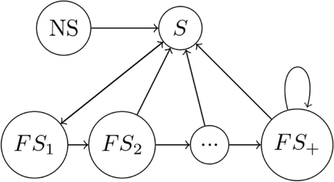
Admissible transitions for smoking substates
Regarding physical activity, we use a binary classification between active and sedentary subjects and let \(\mathcalA=\\textact,\textsed\\), in line with the literature [17] (Fig. 3). Therefore, the condition of each subject is determined by a vector \((e,g,s,a,h)\).
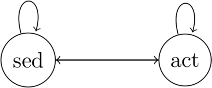
Admissible transitions for physical activity substates
Markov chain initialization
We initialize the cohort based on data from the Italian population in 2019. Let \(P_s,a,h^e,g\) denote the number of subjects of type \((e,g)\) in state \((s,a,h)\). Whenever some indexes among \(s\), \(a\) and \(h\) are missing, a marginalization is implicit, e.g., \(P_a^e,g=\sum _s\in \mathcalS\sum _h\in \mathcalHP_s,a,h^e,g\) indicates the number of subjects of type \((e,g)\) in physical activity substate \(a,\) independently of \(s\) and \(h.\) Due to the lack of joint distribution of health and risk factor states, we make an independence assumption, namely we assume
$$P_s,a,h^e,g\propto P_s,a^e,g\cdot P_h^e,g.$$
The type distribution \(P^e,g\) is derived from [27] and the joint distribution of smoking and physical activity substates \(P_s,a^e,g\) is derived from [28]. The dataset provides a classification in current smokers, former smokers and nonsmokers. Details on the distribution of former smokers by time since cessation are reported in Appendix 1. The distribution of health substate \(P_h^e,g\) is derived from GBD [1], which does not provide the disease joint prevalence. For this reason, we make an additional independence assumption, i.e., we assume that the joint prevalence of multiple diseases is proportional to the product of the single disease prevalence (see Table 2 for details).
Transition probabilities
We let \(\mathrm Q_\left(\mathrm s,\mathrm a,\mathrm h\right),\left(\mathrm s’,\mathrm a’,\mathrm h’\right)^\mathrm e,\mathrm g\) denote the transition probability from state \((\texts,\texta,\texth)\) to state \(\left(\mathrm s’,\;\mathrm a’,\;\mathrm h’\right)\) for a subject of type \(\left(\texte,\textg\right)\), which we factorize by
$$\mathrm Q_\left(\mathrm s,\mathrm a,\mathrm h\right),\left(\mathrm s’,\mathrm a’,\mathrm h’\right)^\mathrm e,\mathrm g=\mathrm Q_\mathrm s,\mathrm s’^\mathrm e,\mathrm g\cdot\mathrm Q_\mathrm a,\mathrm a’^\mathrm e,\mathrm g\cdot\mathrm Q_\mathrm h,\mathrm h’^\mathrm e,\mathrm g\left(\mathrm s,\mathrm a\right).$$
We refer to Table 2 for more details. For every subject, the transition probability matrix describing the smoking substate \(\mathrm Q_\mathrm s,\mathrm s’^\mathrm e,\mathrm g\) and physical activity substate \(\mathrm Q_\mathrm a,\mathrm a’^\mathrm e,\mathrm g\) are independent of the other substates, e.g., the health state of a subject does not influence the behavior related to risk factors. Instead, the transition probabilities in the health state space \(\mathrm Q_\mathrm h,\mathrm h’^\mathrm e,\mathrm g\left(\mathrm s,\mathrm a\right)\) depend on the risk factors exposure, to capture the correlation between risk factors and health, which is the core of the model.
Smoking and physical activity transitions
The transitions between smoking substates follow these rules:
-
Non-smokers cannot become smokers, as it is very unlikely to start smoking for subjects older than 25 [29].
where for males \(A=1.177, B=0.150\), and for females \(A=1.197, B=0.113\) [31].
Due to lack of reliable data, we construct the transition probability that describes the evolution of physical activity substates by requiring that for every type \((e,g)\) the fraction of active and sedentary subjects is constant in time, so that the physical activity transition matrix depends on age. For details, see Appendix 2.
Health transitions
Transitions in the health subspace are distinguished into two classes. The first class describes the probability of getting ill with a tracing disease, which depends on the subject type \((e,g)\) and on her exposure to risk factors \((s,a)\). We introduce the following notation.
-
\(\beta _s,a,m ^e,g\) denotes the probability for a subject of type \((e,g)\) and risk factor substate \((s,a)\) of getting ill with disease \(m\). For simplicity of notation, we let \(\beta _m ^e,g\) denote the probability for a nonsmoker and active subject.
-
\(RR_s,a,m^e,g\) denotes the relative risk (RR) for disease \(m\) for a subject of type \((e,g)\) with exposure to risk factors \((s,a)\) in comparison to nonexposed, i.e.,
$$\beta _s,a,m^e,g=\beta _m^e,g\cdot RR_s,a,m^e,g.$$
(1)
Furthermore, we assume that the RR are obtained additively from the single risk factors, i.e.,
$$RR_s,a,m^e,g=1+(RR_a,m^e,g-1)+(RR_s,m^e,g-1),$$
(2)
where \(RR_a,m^e,g\) and \(RR_s,m^e,g\) indicate the relative risk for sedentary lifestyle and smoking, respectively. The relative risks for sedentary lifestyle and smoking are obtained from [17, 32]. A sensitivity analysis on this assumption is included in the discussion.
-
\(I_m^e,g\) indicates the number of incident cases of disease \(m\) for subjects of type \((e,g)\) in the considered cohort, derived from [1].
The parameters \(\beta _m^e,g\) are derived by imposing that the expected incident cases of disease \(m\) in the first year of the simulation for subjects of type \((e,g)\) coincide with \(I_m^e,g\). To this end, we formulate a relation for the expected number of incident cases. This is obtained as the sum over the states \((s,a,h)\) of the prevalence of subjects in such state (\(P_s,a,h^e,g\)) times the probability of getting ill with disease \(m\) from that state (\(\beta _m^e,gRR_s,a,m^e,g)\). Observe that for subjects ill with disease \(m\) the probability of getting the disease is zero, therefore the sum over the health substates does not include substates \(h\) characterized by disease \(m\). Hence,
$$I_m^e,g=\sum_\beginarraych\in \mathcalH:\\ m\notin h\endarray\sum_s\in \mathcalS\sum_a\in \mathcalAP_s,a,h^e,g\beta _m^e,gRR_s,a,m^e,g.$$
Given \(RR_s,a,m^e,g\), \(P_s,a,h^e,g\), and \(I_m^e,g\), we obtain \(\beta _m^e,g\) by
$$\beta _m^e,g=\fracI_m^e,g\sum_\beginarraych\in \mathcalH:\\ m\notin h\endarray\sum_s\in \mathcalS\sum_a\in \mathcalAP_s,a,h^e,gRR_s,a,m^e,g.$$
Given \(\beta _m^e,g\), we then obtain \(\beta _s,a,m^e,g\) by (1).
The second class of transitions describes the death events. Subjects may die because of tracing diseases or because of other causes. We classify the tracing diseases into two categories: lethal diseases (STR and IHD) and nonlethal disease (LC, COPD, DIA), where by lethal we mean that a large fraction of subjects that suffer from the disease die immediately after the incidence of the disease. The mortality probabilities are calibrated by using similar arguments as before. For details, see Appendix 3.
Simulations and output
The previous sections described the initialization of the Markov chains and the model structure. We now describe the simulation setting. For every time \(t\), we compute by standard results of Markov chains the expected number of subject in every state \((s,a,h)\) for every type \((e,g)\), denoted by \(P_s,a,h^e,g(t)\), via
$$P_s,a,h^e,g\left(t+1\right)=\sum\nolimits_s’,a’,h’P_s’,a’,h’^e-1,g\left(t\right);\mathrmQ_\left(\mathrms’,a’,h’\right),\left(\mathrms,a,h\right)^\mathrme,g+b_s,a,h^e,g\left(t+1\right),$$
where\(b_s,a,h^e,g(t+1\)) denotes the new subjects that are introduced in the population at each time-step. In our simulations the population of new subjects is assumed to be constant in time and composed of subjects with minimal age, with distribution equal to the initial distribution of the population, i.e., \(b_s,a,h^25,g\left(t+1\right)= P_s,a,h^25,g\left(0\right)\) for every time \(t\) and \(b_s,a,h^e,g\left(t+1\right)=0\) for every \(e>25\). However, this can be modified to include time-varying inputs of new subjects, or assuming \(b_s,a,h^e,g\left(t+1\right)=0\) to simulate a closed cohort of subjects. The expected population distribution at each time step allows to compute many quantities of interest (including incident cases, prevalent cases, and deaths for every tracing disease, as well as joint prevalence of tracing diseases and risk factors). Among those, we mention the following ones:
-
YLL (years life lost). Let \(l_g(e)\) denote the life expectation of a subject of type \((e,g)\), derived from the Istat dataset [27]. Given the number of subjects who died in one year for every type \((e,g)\) (denoted by \(D_tot^e,g\)), the corresponding amount of YLL is
$$YLL=\sum_e\in \mathcalE\sum_g\in \mathcalGD_tot^e,g(l_g(e)-e).$$
-
YLD (years lived with disability). A weight \(w_m^e,g\) that measures the impact of disability of each disease \(m\) for subjects of every type \((e,g)\) is derived from [1]. Let \(N_m^e,g\) denote the number of subjects of type \((e,g)\) with disease \(m\). Then,
$$YLD=\sum_e\in \mathcalE\sum_g\in \mathcalG\sum_m\in \mathcalMN_m^e,g\cdot w_m^e,g.$$
-
DALY. These are equal to the sum of YLL and YLD.
We conduct simulations in two different scenarios: baseline scenario and intervention scenario. The effects of an intervention are measured in terms of difference in DALYs between baseline and intervention scenarios. Interventions modify the prevalence of risk factors \(P_s,a^e,g\left(0\right)\) in the targeted population groups at the beginning of the simulation. After the intervention, active subjects are allowed to become sedentary, and former smokers are allowed to relapse smoking, according to the transition probabilities described in “Methods” section. The time horizon of the simulation is arbitrary and the simulation can be conducted either in an open cohort setting or in a closed cohort setting. Since the model does not keep track of prevalent cases of nontracing diseases, to compute the YLD for other causes avoided in the intervention scenario, we assume that the ratio between avoided YLD for other causes and avoided YLD for tracing diseases is equal to the ratio in the baseline scenario.
Uncertainty
The outputs of the model are affected by the parameters’ uncertainty. The impact of the uncertainty of the parameters has been analyzed from a theoretical perspective in [33]. Such an analysis has shown that, among the model parameters, only the relative risks satisfy the following two requirements: they are affected by large uncertainty; the results of the model are very sensitive to them. The uncertainty of our results is obtained by using the confidence limits of literature’s RRs computed with significance level determined by the Bonferroni method assuring an overall confidence of 95%. The Bonferroni method is known to be a very conservative approach, hence estimating the uncertainty based on Montecarlo sampling of the parameters would provide more realistic confidence intervals. On the other hand, the latter approach would require a very large bunch of simulations since the relative risks are hundreds of independent parameters that characterize the increasing risk of subjects exposed to the risk factors for different age, gender and tracing diseases.
link


