IoT-based bed and ventilator management system during the COVID-19 pandemic

IoT-based bright pulse oximeter: A physician can track a patient remotely using an oximeter connected to an Internet of Things (IoT) device. This acts as a real-time warning system that can warn patients if they’re in danger. IoT-based body temperature measurement device (temperature sensor): The unit is small and convenient, and it runs on a 3.3 V battery cell.

We can forecast a time series using the ARIMA model by looking at the past values of the series. A time series is a set of measurements taken at regular intervals. Forecasting is the next step in the process, and it involves predicting the series’ future values. The fundamental business planning, sourcing, and development activities are all guided by forecasting²⁴. Any forecasting errors can affect the entire supply chain or any business context. As a result, it’s essential to get the predictions right to save money and achieve success. A time series can now be divided into two forms of forecasting²⁵. Univariate Time Series Forecasting is when you use only the past values of a time series to estimate future matters. Multi-Variate Time Series Forecasting is when you use predictors other than the series (also known as exogenous variables) to forecast. ARIMA, which stands for “Auto-Regressive Integrated Moving Average,” is a classification method that “explains” a particular time series based on its previous values, i.e., its hick-ups and stagnated. Prediction error, results in an equation that can be used to forecast future information. An ARIMA model is represented by 3 terms: a, b, and c. Where a= the AR term’s sequence, b= the MA term’s sequence and c= the number of differences that must be present in order for the time series to become stationary.

A pure Auto Regressive (AR only) model is one in which X_t is solely determined by its own lags. X_t, in other words, is a feature (or function) of the lags of X′t.

where X_t1 is the series’ lag1, β is the lag1 coefficient calculated by the model, and α is the intercept term estimated by the model.

A pure Moving Average (MA only) model, on the other hand, is one in which X_t is solely determined by the lagged forecast errors.

The errors of the autoregressive models of the corresponding lags are represented by the error terms. The errors ε_t and ε_t−1 are the results of the Equations (3) and (4).

AR and MA were the models of the ARIMA. So here’s what an ARIMA model’s equation looks like. An ARIMA model is one in which the time series has been differenced at least once to make it stationary, and the AR and MA terms have been combined. The equation is presented in Equation (5).

The second model, which has been utilized for predicting future patient admissions, has been computed and analyzed using the Transformer model. The implementation process has been systematically carried out, ensuring that the model’s parameters and configurations are optimized for accurate predictions. Furthermore, the effectiveness of the Transformer model has been evaluated based on its ability to process sequential data and capture complex patterns within the dataset. It has the following layers:

• Data preparation and embeddings The original Transformer design relies on embeddings to represent discrete tokens. For a time-series application, numerical values are normalized and then projected into a continuous embedding space. A linear transformation is frequently used to map each time-step value into an embedding vector. Positional information, which is critical for sequence modeling, is preserved by adding positional encodings. These encodings impose an ordering on the input data, ensuring that temporal relationships are recognized by the model.

• Encoder module The encoder is composed of multiple layers, each containing a multi-head self-attention mechanism and a position-wise feed-forward network. Within each encoder layer, self-attention computes the relevance of each time step to every other time step in the input sequence. This operation is facilitated by query, key, and value projections, which are combined to form attention scores. Multi-head attention extends this process by allowing multiple sets of projections to capture different types of temporal dependencies simultaneously. After the attention sublayer, a feed-forward network is applied to each embedding vector independently. Residual connections and normalization are included to stabilize training and retain information from earlier layers.

• Decoder module (Adapted for Regression) In a standard Transformer, the decoder generates outputs step by step for language modeling tasks. For time-series regression, the decoder can be configured to receive a shifted version of the target sequence (e.g., previous time steps or placeholder values) to predict subsequent values. The decoder follows a structure similar to the encoder but incorporates an additional cross-attention mechanism. This mechanism uses the encoder outputs as keys and values while the decoder states serve as queries, allowing the model to focus on relevant information from the encoded sequence. The final output is often produced by a linear layer that maps the decoder’s hidden states to numeric predictions rather than discrete tokens.

• Training objective Since the goal involves predicting continuous patient counts, a regression loss function such as mean squared error or mean absolute error is employed. Backpropagation is used to adjust the parameters within the encoder-decoder blocks, including attention weights, feed-forward layers, and embedding transformations. Gradient-based optimization algorithms, such as Adam, are commonly utilized to achieve stable convergence.

• Temporal attention and long-range dependencies A primary advantage of this architecture lies in its ability to capture long-range dependencies without relying solely on recurrent connections. By computing attention scores across all time steps simultaneously, the model can learn complex temporal relationships in patient count data, which may include seasonal trends or abrupt changes. Multi-head attention further refines these relationships by enabling the model to attend to different aspects of the sequence in parallel.

• Inference and forecast generation Once the model has been trained, forecast values are produced by feeding the most recent observed data (or previously predicted outputs) into the encoder-decoder structure. The decoder iteratively predicts subsequent time steps until the desired forecast horizon is reached. In practice, teacher forcing or scheduled sampling can be applied during training to balance stability and predictive accuracy. The transformer model architecture has been discussed in the result section.

Proposed model and algorithms

The world’s current COVID-19 pandemic requires a patient safety policy that places a greater focus on epidemiology, particularly identifying effective population-based developmental and learning programs and addressing the consequences²⁶. The healthcare facilities and programs are still in the early stages of growth, with skill shortages, sickness absence, insufficient facilities, and low-quality care among the challenges^27,28. Even though the government’s determination and the National Health Mission, sufficient and sustainable healthcare remains a mirage²⁹. The rural healthcare system is beset by a persistent shortage of medical practitioners, which negatively affects the overall accessibility of care for rural residents³⁰. In certain places, the healthcare infrastructure is insufficient or unprepared to deal with the pandemic like COVID-19 transmission^31,32. To deal with such issues^33,34 and to solve the problem, the proposed scheme has been implemented in this research paper.

The utilization of IoT devices significantly contributed to patient monitoring during the COVID-19 pandemic. Smart sensors were employed to continuously measure vital health parameters such as body temperature, oxygen levels, heart rate, and respiratory function. Data collected through wearable devices and remote monitoring systems were transmitted to healthcare professionals, enabling timely medical responses. By facilitating remote assessments, these technologies helped reduce direct patient contact, thereby lowering the risk of virus transmission and their will not be any direct contacts with the patients. Cloud-based platforms were used for data storage and analysis, supporting predictive insights and early detection of health deterioration. AI-driven algorithms were integrated into IoT systems to identify irregularities and notify medical personnel, ensuring swift intervention. Additionally, automated medication dispensers and intelligent inhalers were implemented to enhance treatment adherence. IoT-enabled tracking mechanisms further assisted in contact tracing and monitoring quarantine compliance. As a result, hospital resources were effectively managed, and patient care was significantly enhanced throughout the pandemic³⁵.

Figure 1 depicts the architecture of the IoT-based healthcare management system for the benefit of the patients and as well as for the hospital management system. Here the patient’s health is being monitored using the body area sensor network. For the sake of simplicity, only parameters are being considered here, i.e., the patients’ body temperature and oxygen level through the IoT devices. This information is then passed to the Local Process Unit (LPU). After that, the data is passed via the Internet to the various stakeholders of the healthcare management systems, such as such emergency ward, physician, and care center of the BSN, where the parameters related to the patient’s details are maintained and observed for any credulity of the patients.

Architecture of the proposed IOT-BVM scheme.

The illustrated architecture is composed of several layers, each intended to manage patients who use IoT devices during the COVID-19 period. In the first layer, body sensors are placed on individuals to collect vital signs. The readings are then received and filtered by a local processing unit. Next, the data are transferred via the internet to a central repository, where they are stored in a database. Critical cases are flagged, and positive results are tracked automatically. This information is then shared with healthcare services, such as emergency departments, physicians, and care centers, to enable ongoing monitoring.

One notable advantage of this layered design is its ability to provide real-time updates on patient health, which supports faster intervention and more informed clinical decisions. In addition, the need for in-person visits can be reduced, lowering the potential for virus transmission. The architecture can also be scaled up if the number of patients increases, offering flexibility in times of high demand. However, certain drawbacks must be acknowledged. A reliable internet connection is required for seamless data flow, and any disruption can affect timely updates. Moreover, patient privacy must be protected through robust data security measures³⁶. Costs related to installing and maintaining sensors, databases, and other infrastructure can also be considerable. Despite these challenges, the layered approach continues to offer valuable support for remote patient care and broader public health initiatives. Fig. 1 shows the architecture of the proposed IOT-BVM scheme.

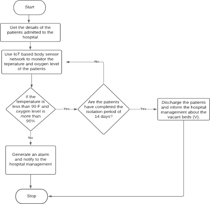
The working of the proposed scheme, IOT-BVM, is expressed in flowcharts 1 and 2. Figure 2 depicts the working mechanism of flowchart 1 and the operations of the process that is being undergone inside the hospital management. Initially, the details of the patients are identified who are presently admitted to the hospital. The patients are being monitored using the IoT-based environment, and it is being checked whether or not the temperature and oxygen level are in the correct range. If it’s not proper, continuous monitoring will be done.

Flowchart of the proposed system.

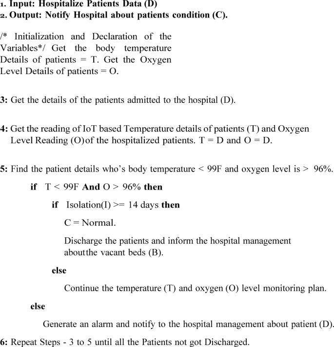
If the monitored information results in the details that indicate that the patients are being recovered and if they have completed the 14 days of the isolation period, then they are to be in the process of getting discharged from the hospital, and its information must be passed to the stakeholders of the hospital system. The outcome of this algorithm is 1 the total number of available beds and is denoted as “V”, The algorithm 1 represents herein.

The time complexity of the algorithm 1 can be analyzed by looking at the steps involved in the procedure. Let n represent the number of hospitalized patients. In Step 3, retrieving the details of the patients is a constant-time operation, O(1), since it’s just an input data retrieval. In Step 4, fetching the IoT-based body temperature (T) and oxygen level readings (O) for each patient requires iterating through each patient’s data. This operation takes O(n) time, where nn is the number of patients, because it involves fetching and storing data for all patients. Step 5 consists of checking each patient’s body temperature and oxygen level. The comparison of these values is a constant-time operation, O(1), for each patient. If a patient meets the specified conditions (temperature < 99°F and oxygen level > 96%), the algorithm either discharges the patient or continue’s monitoring based on whether the isolation period has passed. This decision-making process also takes constant time, O(1), per patient. If the conditions are not met, an alarm is generated and the hospital management is notified, which is again an O(1) operation. Since these steps are executed for each patient, Step 5 has a time complexity of O(n). Finally, Step 6 involves repeating the evaluation process until all patients are discharged. Since each patient is processed only once, the overall time complexity of this loop remains O(n). Thus, considering all steps together, the total time complexity of the algorithm is O(n), where nn is the number of hospitalized patients. This indicates that the algorithm’s execution time increases linearly with the number of patients, making it a highly efficient solution for managing patient data in real time.

The system performance of this algorithm can be evaluated based on its efficiency, responsiveness, and scalability. In terms of efficiency, the algorithm performs well because it operates in linear time, O(n). Each step of the procedure involves essential operations, such as retrieving data, comparing patient conditions, and triggering the necessary actions based on those comparisons. As the number of patients increases, the system’s performance remains proportional to the data size, making it well-suited for managing larger datasets without excessive delays. Regarding responsiveness, the algorithm is designed to make decisions promptly. It evaluates each patient’s condition and, based on the results, either discharges the patient, continues monitoring, or raises an alarm. This ensures that the hospital management system can respond quickly to any changes in a patient’s condition, improving patient care and hospital workflow. The ability to react immediately is crucial for real-time healthcare applications, where fast decision-making can directly impact patient outcomes.

In terms of scalability, the algorithm is capable of handling an increasing number of patients without significant performance degradation. Since the time complexity is linear, the system scales efficiently with the number of patients. For very large datasets, the processing time will increase proportionally, but the algorithm will still function adequately as long as the hospital’s infrastructure is equipped to manage the additional data. Finally, in terms of resource utilization, the algorithm relies mainly on data retrieval and condition checks, both of which are low-complexity operations. This results in minimal resource consumption, making the system efficient in terms of CPU and memory usage. However, as the dataset grows, additional infrastructure might be needed to handle the increased data processing load. Hence, the algorithm offers efficient performance with linear time complexity, ensuring that it can handle the increasing scale of patient data without significant delays. Its quick decision-making process enhances responsiveness, and its scalability makes it suitable for use in larger hospitals or healthcare facilities. Overall, the system is designed to perform effectively in real-time environments, balancing efficiency, scalability, and resource usage.

The procedure inside the hospital.

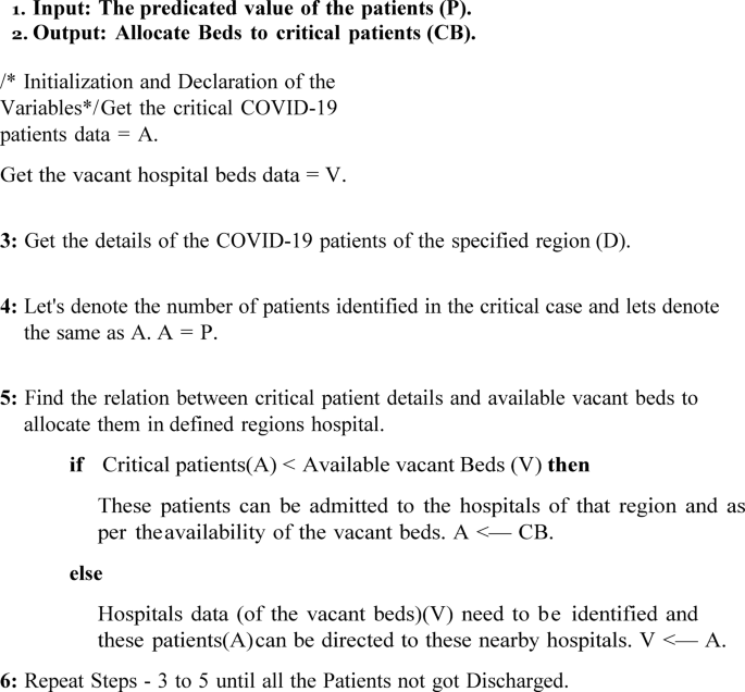
Flowchart 2 is the subpart of the proposed scheme and is represented in Fig. 3. Figure 3 depicts the scenario where the comparison of the available beds (V) and the positive cases and its prediction of the Confirmed cases (A) are taken into consideration in that particular region. Then this is compared to get the idea that the vacant beds are available in enough away so that the patients can be admitted and will be given good services by the healthcare systems. In case the available beds are not present, then the nearby hospital vacancies beds data is to be identified so that the patients can be accommodated in the hospitals; the same is depicted in Algorithm 2.

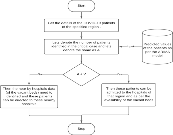
Flowchart depicting the process inside the hospital and the confirmed cases around the same region.

The procedure inside the hospital and the positive cases around the same region.

The outcome of the mentioned approach solves the problem of managing the patients in this pandemic situation. The services can be improved as the data will be available in advance, and the hospital management will have enough time to arrange the physicians, medical devices, staff, and vacant beds. This will also aid the healthcare systems to be prepared in advance with the availability of medical equipment. The following section discusses the performance evaluations of the proposed scheme.

The time complexity of the algorithm 2 can be analyzed by evaluating the operations involved in each step. Let n represent the number of critical COVID-19 patients and mm represent the number of available vacant beds in the region. In Step 3, retrieving the details of the COVID-19 patients for a specified region is an O(1) operation, assuming the data is readily available. Step 4 involves assigning the number of critical patients (denoted as A) from the retrieved data, which is a simple assignment and thus takes constant time, O(1). In Step 5, the algorithm compares the number of critical patients A with the available vacant beds VV. This comparison is a constant-time operation, O(1). If the number of critical patients is less than the available beds, the algorithm allocates beds by admitting the patients to hospitals in the region, which again takes constant time, O(1). However, if the number of critical patients exceeds the available beds, the algorithm needs to identify hospitals with vacant beds, which requires scanning the list of hospitals. This step takes O(m) time, where mm is the number of hospitals. Once the hospitals with available beds are identified, assigning patients to these hospitals takes O(1) per patient. Finally, Step 6 involves repeating the process until all patients are discharged. Since each patient is evaluated once, this loop runs O(n) times. Given that the algorithm may require scanning all hospitals in the worst case, the overall time complexity of the algorithm is O(n⋅m), where n is the number of critical patients and mm is the number of hospitals. This time complexity suggests that as the number of critical patients and hospitals increases, the algorithm’s execution time will scale accordingly.

The system performance of this algorithm can be assessed in terms of efficiency, responsiveness, and scalability. In terms of efficiency, the algorithm performs well for smaller datasets, as most operations are constant-time, O(1), including retrieving data and assigning patients to hospitals. The primary area where performance may degrade is when identifying hospitals with available beds, which requires scanning the list of hospitals. As the number of hospitals grows, this step can become a bottleneck, increasing the overall time complexity to O(n⋅m). Therefore, while the algorithm is efficient for smaller datasets, its performance may decrease with a larger number of hospitals or patients. In terms of responsiveness, the algorithm ensures quick decision-making when allocating beds to critical patients. If the number of critical patients is less than the number of vacant beds, they can be admitted to the available hospitals in the region, which ensures that patients are admitted promptly. If there are more critical patients than vacant beds, the algorithm identifies nearby hospitals with available beds and directs patients accordingly. This ensures that the system is responsive and that no critical patient is left without attention, making it highly suitable for real-time applications in healthcare settings.

Regarding scalability, the algorithm can handle a growing number of patients, but its scalability is affected by the number of hospitals in the region. As the number of hospitals increases, the algorithm’s performance may suffer due to the need to scan a larger list of hospitals for available beds. This means that while the algorithm is scalable to a degree, it may require optimizations, such as indexing hospitals or clustering them based on location or availability, to improve efficiency when the number of hospitals or patients grows significantly. Lastly, in terms of resource utilization, the algorithm is generally efficient, as it primarily performs basic comparisons and assignments. However, the process of identifying vacant beds in hospitals can be resource-intensive, especially if the list of hospitals is large. As the dataset grows, the system may need more resources to manage the increased computational load. Therefore, the algorithm is suitable for smaller-scale applications, but for larger datasets, it might require infrastructure improvements or optimization techniques to ensure optimal performance. Hence, while the algorithm offers an efficient and responsive solution for allocating beds to critical patients, its time complexity of O(n⋅m) makes it less efficient as both the number of patients and hospitals increases. The system performs well for smaller datasets but may face challenges with scalability and resource usage when handling larger volumes of data. To ensure better performance at scale, optimizations such as data indexing or improved searching algorithms could be considered.